flowchart TD A(Key Variables Used \n event_id_cnty) A --> B(Time Period) A --> C(Characteristic of Incident) A --> D(Location) B --> E(year) B --> F(date) C --> K(event_type) C --> L(sub_event_type) C --> M(actor1) C --> N(actor2) C --> O(fatalities) C -.-> P(New Variables) P -.-> Q(total incidents) P -.-> R(total fatalities) P -.-> S(political violence rate) P -.-> T(violence against civilian rate) D --> U(country) D --> V(longitude) D --> W(latitude) D --> X(admin1) D --> Y(admin2) D --> Z(admin3) D -.-> AA(New Variables) AA -.-> AB(geometry points) AA -.-> AC(shapeID)
Take-home Exercise 4 - Part 2
Decoding Chaos: Geospatial Data Exploratory Analysis (GDEA)
1. Overview
Note: This is a continuation of the take-home exercise 4.
This assignment is separated into three segments (web pages):
1. Initial Data Exploratory Analysis (IDEA) – Click here for IDEA page.
2. Geospatial Data Exploratory Analysis (GDEA) – Current Page
3. Prototype: Exploratory – Click here for Prototype: Exploratory page..
2. Geospatial Data Preparation
The flowchart diagram below provides an overview of the key variables used for geospatial data exploration.
2.1 Install and launch R packages
The project uses p_load() of pacman package to check if the R packages are installed in the computer.
The following code chunk is used to install and launch the R packages.
Show code
pacman::p_load(tidyverse, kableExtra, knitr,
sf, spdep, tmap, leaflet, leaflet.extras,
tm, plotly)2.2 Import Aspatial Data
This section will import the dataset from Initial Data Exploratory Analysis segment. Original dataset is retrieved from Armed Conflict Location & Event Data Project (ACLED), specifically Myanmar country, between Year 2010 and Year 2023.
final <- readRDS("data/final.rds")EPSG:4979 is WGS 84 Geographic Coordinate system and EPSG:4144 is Myanmar Projected Coordinate System will be used.
Convert listing data frame to simple feature dataframe
Use st_as_sf() from sf package to convert listing data frame into simple feature data frame.
coordsargument requires the columns of x-and-y-coordinates.crsargument requires the coordinates system in epsg format.
Show code
data_sf4144 <- st_as_sf(final,
coords = c("longitude", "latitude"),
crs=4979) %>%
st_transform(crs = 4144)Show code
write_rds(data_sf4144,
"data/myan.rds")Verify projection of newly transformed data_sf
Use st_crs() to verify the projection of the newly transformed data_sf.
The output below shows that the EPSG is indicated as 4144, which is the correct format for Myanmar.
Show code
st_crs(data_sf4144)Coordinate Reference System:
User input: EPSG:4144
wkt:
GEOGCRS["Kalianpur 1937",
DATUM["Kalianpur 1937",
ELLIPSOID["Everest 1830 (1937 Adjustment)",6377276.345,300.8017,
LENGTHUNIT["metre",1]]],
PRIMEM["Greenwich",0,
ANGLEUNIT["degree",0.0174532925199433]],
CS[ellipsoidal,2],
AXIS["geodetic latitude (Lat)",north,
ORDER[1],
ANGLEUNIT["degree",0.0174532925199433]],
AXIS["geodetic longitude (Lon)",east,
ORDER[2],
ANGLEUNIT["degree",0.0174532925199433]],
USAGE[
SCOPE["Geodesy."],
AREA["Bangladesh - onshore; India - mainland onshore; Myanmar - onshore and Moattama area offshore; Pakistan - onshore."],
BBOX[8.02,60.86,37.07,101.17]],
ID["EPSG",4144]]View extent of data_sf
Use st_bbox() to view extent of data_sf.
Show code
st_bbox(data_sf4144) xmin ymin xmax ymax
92.201982 9.980644 100.357600 27.731000 2.3 Import Geospatial Data
Myanmar Level-2 Administrative Boundary (also known as Local Government Area, LGA) polygon features GIS data was downloaded from geoBoundaries.
Read geospatial layers
Use st_read to read geospatial layers.
Show code
myan_bound_adm2 <- st_read(dsn="data",
layer="geoBoundaries-MMR-ADM2")Reading layer `geoBoundaries-MMR-ADM2' from data source
`C:\teoose\ISSS608\Take-home_Ex\Take-home_Ex04\data' using driver `ESRI Shapefile'
Simple feature collection with 74 features and 5 fields
Geometry type: MULTIPOLYGON
Dimension: XY
Bounding box: xmin: 92.17275 ymin: 9.671252 xmax: 101.1699 ymax: 28.54554
Geodetic CRS: WGS 84Show code
myan_bound <- myan_bound_adm2# myan_bound_adm1 <- st_read(dsn="data", layer="geoBoundaries-MMR-ADM1")
# myan_bound_adm3 <- st_read(dsn="data", layer="geoBoundaries-MMR-ADM3")glimpse(myan_bound)Rows: 74
Columns: 6
$ shapeName <chr> "Hinthada", "Labutta", "Maubin", "Myaungmya", "Pathein", "P…
$ shapeISO <chr> NA, NA, NA, NA, NA, NA, NA, NA, NA, NA, NA, NA, NA, NA, NA,…
$ shapeID <chr> "60261553B48695999525720", "60261553B3473904040713", "60261…
$ shapeGroup <chr> "MMR", "MMR", "MMR", "MMR", "MMR", "MMR", "MMR", "MMR", "MM…
$ shapeType <chr> "ADM2", "ADM2", "ADM2", "ADM2", "ADM2", "ADM2", "ADM2", "AD…
$ geometry <MULTIPOLYGON [°]> MULTIPOLYGON (((95.2637 18...., MULTIPOLYGON (…Check Coordinate Reference System (CRS) of Myanmar boundary
Use st_crs() to check the set coordinate system of myan_bound.
st_crs(myan_bound)Coordinate Reference System:
User input: WGS 84
wkt:
GEOGCRS["WGS 84",
ENSEMBLE["World Geodetic System 1984 ensemble",
MEMBER["World Geodetic System 1984 (Transit)"],
MEMBER["World Geodetic System 1984 (G730)"],
MEMBER["World Geodetic System 1984 (G873)"],
MEMBER["World Geodetic System 1984 (G1150)"],
MEMBER["World Geodetic System 1984 (G1674)"],
MEMBER["World Geodetic System 1984 (G1762)"],
MEMBER["World Geodetic System 1984 (G2139)"],
ELLIPSOID["WGS 84",6378137,298.257223563,
LENGTHUNIT["metre",1]],
ENSEMBLEACCURACY[2.0]],
PRIMEM["Greenwich",0,
ANGLEUNIT["degree",0.0174532925199433]],
CS[ellipsoidal,2],
AXIS["geodetic latitude (Lat)",north,
ORDER[1],
ANGLEUNIT["degree",0.0174532925199433]],
AXIS["geodetic longitude (Lon)",east,
ORDER[2],
ANGLEUNIT["degree",0.0174532925199433]],
USAGE[
SCOPE["Horizontal component of 3D system."],
AREA["World."],
BBOX[-90,-180,90,180]],
ID["EPSG",4326]]The output above reveals that the EPSG is set at 4326 instead of 4144.
Update CRS information
Use st_transform() to assign correct EPSG code to dataframe, from one coordinate system to another coordinate system mathematically.
myan_bound4144 <- st_transform(myan_bound, 4144)Use st_crs() again to double-check the set coordinate system of myan_bound4144 if it has been set correctly.
st_crs(myan_bound4144)Coordinate Reference System:
User input: EPSG:4144
wkt:
GEOGCRS["Kalianpur 1937",
DATUM["Kalianpur 1937",
ELLIPSOID["Everest 1830 (1937 Adjustment)",6377276.345,300.8017,
LENGTHUNIT["metre",1]]],
PRIMEM["Greenwich",0,
ANGLEUNIT["degree",0.0174532925199433]],
CS[ellipsoidal,2],
AXIS["geodetic latitude (Lat)",north,
ORDER[1],
ANGLEUNIT["degree",0.0174532925199433]],
AXIS["geodetic longitude (Lon)",east,
ORDER[2],
ANGLEUNIT["degree",0.0174532925199433]],
USAGE[
SCOPE["Geodesy."],
AREA["Bangladesh - onshore; India - mainland onshore; Myanmar - onshore and Moattama area offshore; Pakistan - onshore."],
BBOX[8.02,60.86,37.07,101.17]],
ID["EPSG",4144]]The output above reveals that the EPSG is now set correctly to 4144.
2.4 Data Wrangling
Join Aspatial data and Geospatial data
Use st_join() to do a spatial join to related the polygon IDs to each armed conflict incident by its location. Then use join = st_intersects() to identify the points in each LGA.
Show code
joined_data <- st_join(data_sf4144, myan_bound4144,
join = st_intersects,
left = TRUE)Derive number of armed conflicts at each administrative region
Use st_intersect() to identify armed conflicts located within each sub-national administrative region two.
Show code
inci_pts <- myan_bound4144 %>%
mutate(total_inci = lengths(
st_intersects(myan_bound4144, data_sf4144)
))Derive density area at each administrative region
Use st_area() to derive the area of each sub-national administrative region two.
Show code
inci_pts$Area <- inci_pts %>%
st_area()Create new variables
New variables are created at sub-national administrative region two for the years (2010 to 2023).
Annual total fatalities
Annual total armed conflicts
Annual percentage of political violence
Annual percentage of violence against civilian
Show code
for (year in 2010:2023) {
# Filter data_sf4144 for the current year
data_sf4144_year <- data_sf4144[data_sf4144$year == year, ]
# Perform spatial join
joined_data <- st_join(inci_pts, data_sf4144_year)
##############
# Summarise total fatalities at each adm2 level in myan_bound4144
# Replace NA with 0 for polygons with no fatalities
total_fata_col <- paste0('total_fata_', year)
inci_pts[[total_fata_col]] <- tapply(joined_data$fatalities, joined_data$shapeID, sum)
inci_pts[[total_fata_col]][is.na(inci_pts[[total_fata_col]])] <- 0
# Summarise percentage of fatalities at each adm2 level in myan_bound4144
pct_fata_col <- paste0('pct_fata_', year)
inci_pts[[pct_fata_col]] <- round(inci_pts[[total_fata_col]] / sum(inci_pts[[total_fata_col]]) * 100, 2)
inci_pts[[pct_fata_col]][is.na(inci_pts[[pct_fata_col]])] <- 0
##############
# Summarise total incidents at each adm2 level in myan_bound4144
# Replace NA with 0 for polygons with no incidents
total_inci_col <- paste0('total_inci_', year)
inci_pts[[total_inci_col]] <- tapply(joined_data$year, joined_data$shapeID, sum)
inci_pts[[total_inci_col]][is.na(inci_pts[[total_inci_col]])] <- 0
# Summarise percentage of incidents at each adm2 level in myan_bound4144
pct_inci_col <- paste0('pct_inci_', year)
inci_pts[[pct_inci_col]] <- round(inci_pts[[total_inci_col]] / sum(inci_pts[[total_inci_col]]) * 100, 2)
inci_pts[[pct_inci_col]][is.na(inci_pts[[pct_inci_col]])] <- 0
##############
# Summarise total political violence rate at each adm2 level in myan_bound4144
# Replace NA with 0 for polygons with no incidents
total_politicalrate_col <- paste0('total_politicalrate_', year)
inci_pts[[total_politicalrate_col]] <- tapply(joined_data$political_rate, joined_data$shapeID, sum)
inci_pts[[total_politicalrate_col]][is.na(inci_pts[[total_politicalrate_col]])] <- 0
# Summarise percentage of political violence rate at each adm2 level in myan_bound4144
pct_politicalrate_col <- paste0('pct_politicalrate_', year)
inci_pts[[pct_politicalrate_col]] <-
round(inci_pts[[total_politicalrate_col]] / sum(inci_pts[[total_inci_col]]) * 100, 2)
inci_pts[[pct_politicalrate_col]][is.na(inci_pts[[pct_politicalrate_col]])] <- 0
##############
# Summarise total civilian violence rate at each adm2 level in myan_bound4144
# Replace NA with 0 for polygons with no incidents
total_civilianrate_col <- paste0('total_civilianrate_', year)
inci_pts[[total_civilianrate_col]] <- tapply(joined_data$civilian_rate, joined_data$shapeID, sum)
inci_pts[[total_civilianrate_col]][is.na(inci_pts[[total_civilianrate_col]])] <- 0
# Summarise percentage of civilian violence rate at each adm2 level in myan_bound4144
pct_civilianrate_col <- paste0('pct_civilianrate_', year)
inci_pts[[pct_civilianrate_col]] <-
round(inci_pts[[total_civilianrate_col]] / sum(inci_pts[[total_inci_col]]) * 100, 2)
inci_pts[[pct_civilianrate_col]][is.na(inci_pts[[pct_civilianrate_col]])] <- 0
##############
# Summarise by event_type at each adm2 level in myan_bound4144
event_types <- unique(data_sf4144$event_type)
for (event_type in event_types) {
event_count_col <- paste0(event_type, '_', year)
inci_pts[[event_count_col]] <- tapply(joined_data$event_type == event_type, joined_data$shapeID, sum)
inci_pts[[event_count_col]][is.na(inci_pts[[event_count_col]])] <- 0
}
}Use tapply() to perform statistical summaries (such as total fatalities in each region) by group based on selected factors.
Show code
inci_pts$total_fata <-
tapply(joined_data$fatalities, joined_data$shapeID, sum)Filter dataset
The code chunk below to compute density area of total armed conflict incidents and total fatalities at each “second sub-national administrative region” level, and filter the selected variables for subsequent geospatial analysis.
Show code
mapping_rates <- inci_pts %>%
mutate(# density rates
inci_density = as.numeric(`total_inci`/Area * 1000000),
fata_density = as.numeric(`total_fata`/Area * 1000000)) %>%
replace_na(list(inci_density = 0, fata_density = 0, total_fata = 0,
total_inci = 0)) %>%
select(shapeName, shapeID, shapeGroup, shapeType, geometry,
total_inci, inci_density,
total_fata, fata_density, starts_with("pct"))The code chunk below save the cleaned dataset in .rds format for R Shiny Application.
write_rds(mapping_rates,
"data/mapping_rates.rds")3. Geospatial Exploratory Data Analysis
The flowchart diagram below shows an overview of the five geospatial explorations.
flowchart TD A(Geospatial Explorations) A --> B(Spatial Statistical Distribution) A --> C(Spatial Area Density) A --> D(Spatial Distribution) A --> E(Spatial Points) A --> F(Spatial Intensity)
The code chunk below turns R display into plot mode.
tmap_mode("plot")3.1 Spatial Statistical Distribution
To visualise the spatial statistical distribution of armed conflicts at administrative region-levels, the team will use boxmap by creating boxbreak functions. The boxmap is a spatial representation akin to boxplot and histogram, which is useful to detect outliers and visualise distribution of variables.
Create boxbreak function
The code chunk below is a boxmap function that creates break points for a box map.
arguments:
v: vector with observations
mult: multiplier for IQR (default 1.5)
returns:
- bb: vector with 7 break points compute quartile and fences
Show code
boxbreaks <- function(v,mult=1.5) {
qv <- unname(quantile(v))
iqr <- qv[4] - qv[2]
upfence <- qv[4] + mult * iqr
lofence <- qv[2] - mult * iqr
# initialize break points vector
bb <- vector(mode="numeric",length=7)
# logic for lower and upper fences
if (lofence < qv[1]) { # no lower outliers
bb[1] <- lofence
bb[2] <- floor(qv[1])
} else {
bb[2] <- lofence
bb[1] <- qv[1]
}
if (upfence > qv[5]) { # no upper outliers
bb[7] <- upfence
bb[6] <- ceiling(qv[5])
} else {
bb[6] <- upfence
bb[7] <- qv[5]
}
bb[3:5] <- qv[2:4]
return(bb)
}Create get.var function
The code chunk below is an get.var function to extract a variable as a vector out of an sf data frame.
arguments:
vname: variable name (as character, in quotes)
df: name of sf data frame
returns:
- v: vector with values (without a column name)
Show code
get.var <- function(vname,df) {
v <- df[vname] %>% st_set_geometry(NULL)
v <- unname(v[,1])
return(v)
}Create boxmap function
The code chunk below is an boxmap function to create a box map.
arguments:
vnam: variable name (as character, in quotes)
df: simple features polygon layer
legtitle: legend title
mtitle: map title
mult: multiplier for IQR
returns: a tmap-element (plots a map)
Show code
boxmap <- function(vnam, df,
legtitle=NA,
mtitle= paste0("Box Map of ", vnam),
mult=1.5){
var <- get.var(vnam,df)
bb <- boxbreaks(var)
tm_shape(df) +
tm_polygons() +
tm_shape(df) +
tm_fill(vnam,title=legtitle,
breaks=bb,
palette="Reds",
labels = c("lower outlier",
"< 25%",
"25% - 50%",
"50% - 75%",
"> 75%",
"upper outlier")) +
tm_borders() +
tm_layout(main.title = mtitle,
title.position = c("left",
"top"))
}Plot boxmap
The code chunk below uses boxmap() to plot boxmap and tmap_arrange() to arrange small multiple maps in grid layout. Extreme outliers and different quartiles are encoded in different colour intensity, within Myanmar’s geographical area.
Show code
box_inci <- boxmap("total_inci", mapping_rates)
box_fata <- boxmap("total_fata", mapping_rates)
tmap_arrange(box_fata, box_inci, asp=1, ncol=2)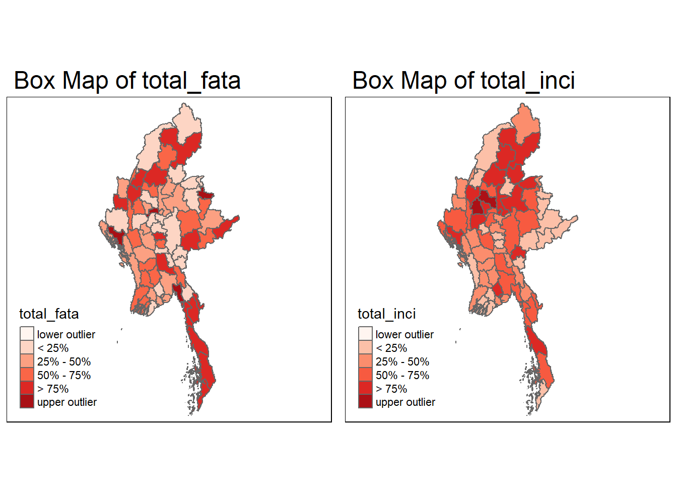
3.2 Spatial Area Density
This segment will visualise spatial area density (concentration) within the different geographical sub-national administrative regions by plotting density map.
Visualising Spatial Density of Armed Conflicts
The code chunk below uses tm_shape() to plot the density map based on the density variables created earlier.
arguments:
style: classification is set to kmeans
n: number of classes is set to 10
Show code
inci_den <- tm_shape(mapping_rates) +
tm_fill("inci_density",
n = 6,
style = "kmeans",
palette = "Reds",
legend.hist = TRUE,
legend.is.portrait = TRUE,
legend.hist.z = 0.1) +
tm_borders(lwd = 0.1,
alpha = 1) +
tm_layout(main.title = "Spatial Density of Armed Conflicts in Myanmar \n(kmeans Classification)",
title = "",
main.title.size = 1,
legend.height = 0.60,
legend.width = 5.0,
legend.outside = FALSE,
legend.position = c("left", "bottom"))
fata_den <- tm_shape(mapping_rates) +
tm_fill("fata_density",
n = 6,
style = "kmeans",
palette = "Reds",
legend.hist = TRUE,
legend.is.portrait = TRUE,
legend.hist.z = 0.1) +
tm_borders(lwd = 0.1,
alpha = 1) +
tm_layout(main.title = "Spatial Density of Fatalities in Myanmar \n(kmeans Classification)",
title = "",
main.title.size = 1,
legend.height = 0.60,
legend.width = 5.0,
legend.outside = FALSE,
legend.position = c("left", "bottom"))Show code
tmap_arrange(inci_den, fata_den,
asp = 1,
ncol=2, nrow=1)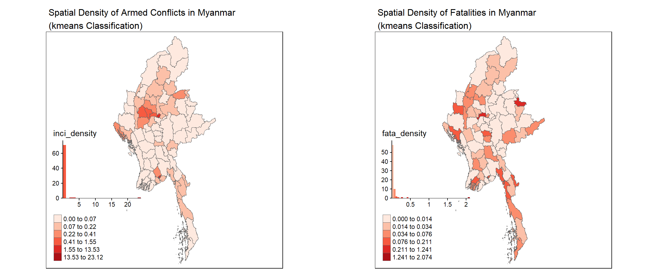
3.3 Spatial Distribution
This segment will visualise spatial pattern or distribution across different geographical subnational administrative regions by plotting choropleth map.
Spatial distribution of armed conflicts
Spatial distribution of political violence
Spatial distribution of violence against civilians
Spatial distribution of fatalities
Visualising Spatial Distribution of Armed Conflicts
The code chunk below uses tm_shape() to plot the maps and tmap_arrange() to arrange small multiple maps in grid layout.
arguments:
style: classification is set to equal, pretty, quantile, kmeans respectively
n: number of classes is set to 6
Distribution of Armed Conflict (by classifications)
Show code
class_equal <- tm_shape(mapping_rates) +
tm_fill("total_inci",
n = 6,
style = "equal",
palette = "Reds",
legend.hist = TRUE,
legend.is.portrait = TRUE,
legend.hist.z = 0.1) +
tm_borders(lwd = 0.1,
alpha = 1) +
tm_layout(main.title = "Distribution of Armed Conflicts in Myanmar \nEqual classification",
title = "(2010-2023)",
main.title.size = 0.7,
legend.height = 0.60,
legend.width = 5.0,
legend.outside = FALSE,
legend.position = c("left", "bottom"))
class_pretty <- tm_shape(mapping_rates) +
tm_fill("total_inci",
n = 6,
style = "pretty",
palette = "Reds",
legend.hist = TRUE,
legend.is.portrait = TRUE,
legend.hist.z = 0.1) +
tm_borders(lwd = 0.1,
alpha = 1) +
tm_layout(main.title = "Distribution of Armed Conflicts in Myanmar \nPretty classification",
title = "(2010-2023)",
main.title.size = 0.7,
legend.height = 0.60,
legend.width = 5.0,
legend.outside = FALSE,
legend.position = c("left", "bottom"))
class_quant <- tm_shape(mapping_rates) +
tm_fill("total_inci",
n = 6,
style = "quantile",
palette = "Reds",
legend.hist = TRUE,
legend.is.portrait = TRUE,
legend.hist.z = 0.1) +
tm_borders(lwd = 0.1,
alpha = 1) +
tm_layout(main.title = "Distribution of Armed Conflicts in Myanmar \nQuantile classification",
title = "(2010-2023)",
main.title.size = 0.7,
legend.height = 0.60,
legend.width = 5.0,
legend.outside = FALSE,
legend.position = c("left", "bottom"))
class_kmeans <- tm_shape(mapping_rates) +
tm_fill("total_inci",
n = 6,
style = "kmeans",
palette = "Reds",
legend.hist = TRUE,
legend.is.portrait = TRUE,
legend.hist.z = 0.1) +
tm_borders(lwd = 0.1,
alpha = 1) +
tm_layout(main.title = "Distribution of Armed Conflicts in Myanmar \nKmeans classification",
title = "(2010-2023)",
main.title.size = 0.7,
legend.height = 0.60,
legend.width = 5.0,
legend.outside = FALSE,
legend.position = c("left", "bottom"))Show code
tmap_arrange(class_equal, class_pretty, class_quant, class_kmeans, asp=1, ncol=4) 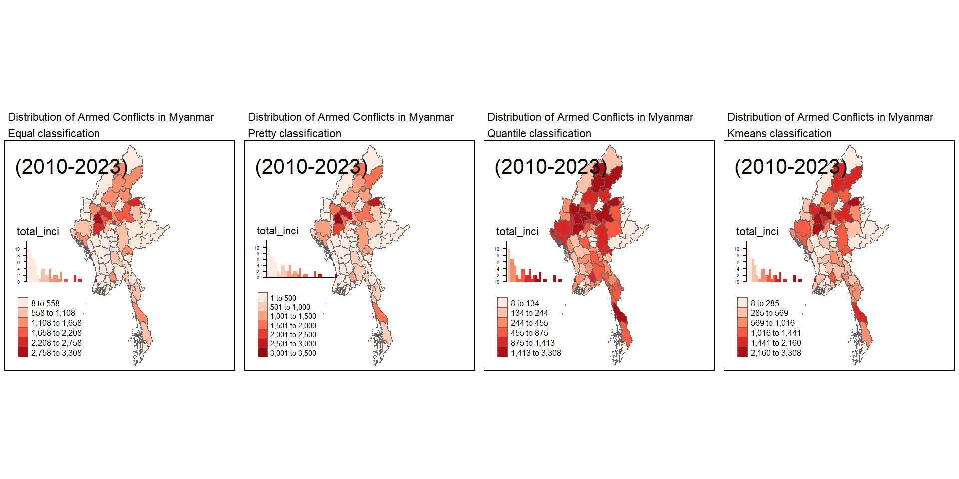
Spatial Distribution of Political Violence (2010 to 2023)
Show code
pv10 <- tm_shape(mapping_rates) +
tm_fill("pct_politicalrate_2010",
n = 6,
style = "kmeans",
palette = "Reds",
legend.hist = TRUE,
legend.is.portrait = TRUE,
legend.hist.z = 0.1) +
tm_borders(lwd = 0.1,
alpha = 1) +
tm_layout(main.title = "Spatial Distribution of Political Violence \nin Myanmar (kmeans Classification)",
title = "2010",
main.title.size = 0.55,
legend.height = 0.60,
legend.width = 5.0,
legend.outside = FALSE,
legend.position = c("left", "bottom"))
pv11 <- tm_shape(mapping_rates) +
tm_fill("pct_politicalrate_2011",
n = 6,
style = "kmeans",
palette = "Reds",
legend.hist = TRUE,
legend.is.portrait = TRUE,
legend.hist.z = 0.1) +
tm_borders(lwd = 0.1,
alpha = 1) +
tm_layout(main.title = "Spatial Distribution of Political Violence \nin Myanmar (kmeans Classification)",
title = "2011",
main.title.size = 0.55,
legend.height = 0.60,
legend.width = 5.0,
legend.outside = FALSE,
legend.position = c("left", "bottom"))
pv12 <- tm_shape(mapping_rates) +
tm_fill("pct_politicalrate_2012",
n = 6,
style = "kmeans",
palette = "Reds",
legend.hist = TRUE,
legend.is.portrait = TRUE,
legend.hist.z = 0.1) +
tm_borders(lwd = 0.1,
alpha = 1) +
tm_layout(main.title = "Spatial Distribution of Political Violence \nin Myanmar (kmeans Classification)",
title = "2012",
main.title.size = 0.55,
legend.height = 0.60,
legend.width = 5.0,
legend.outside = FALSE,
legend.position = c("left", "bottom"))
pv13 <- tm_shape(mapping_rates) +
tm_fill("pct_politicalrate_2013",
n = 6,
style = "kmeans",
palette = "Reds",
legend.hist = TRUE,
legend.is.portrait = TRUE,
legend.hist.z = 0.1) +
tm_borders(lwd = 0.1,
alpha = 1) +
tm_layout(main.title = "Spatial Distribution of Political Violence \nin Myanmar (kmeans Classification)",
title = "2013",
main.title.size = 0.55,
legend.height = 0.60,
legend.width = 5.0,
legend.outside = FALSE,
legend.position = c("left", "bottom"))
pv14 <- tm_shape(mapping_rates) +
tm_fill("pct_politicalrate_2014",
n = 6,
style = "kmeans",
palette = "Reds",
legend.hist = TRUE,
legend.is.portrait = TRUE,
legend.hist.z = 0.1) +
tm_borders(lwd = 0.1,
alpha = 1) +
tm_layout(main.title = "Spatial Distribution of Political Violence \nin Myanmar (kmeans Classification)",
title = "2014",
main.title.size = 0.55,
legend.height = 0.60,
legend.width = 5.0,
legend.outside = FALSE,
legend.position = c("left", "bottom"))
pv15 <- tm_shape(mapping_rates) +
tm_fill("pct_politicalrate_2015",
n = 6,
style = "kmeans",
palette = "Reds",
legend.hist = TRUE,
legend.is.portrait = TRUE,
legend.hist.z = 0.1) +
tm_borders(lwd = 0.1,
alpha = 1) +
tm_layout(main.title = "Spatial Distribution of Political Violence \nin Myanmar (kmeans Classification)",
title = "2015",
main.title.size = 0.55,
legend.height = 0.60,
legend.width = 5.0,
legend.outside = FALSE,
legend.position = c("left", "bottom"))
pv16 <- tm_shape(mapping_rates) +
tm_fill("pct_politicalrate_2016",
n = 6,
style = "kmeans",
palette = "Reds",
legend.hist = TRUE,
legend.is.portrait = TRUE,
legend.hist.z = 0.1) +
tm_borders(lwd = 0.1,
alpha = 1) +
tm_layout(main.title = "Spatial Distribution of Political Violence \nin Myanmar (kmeans Classification)",
title = "2016",
main.title.size = 0.55,
legend.height = 0.60,
legend.width = 5.0,
legend.outside = FALSE,
legend.position = c("left", "bottom"))
pv17 <- tm_shape(mapping_rates) +
tm_fill("pct_politicalrate_2017",
n = 6,
style = "kmeans",
palette = "Reds",
legend.hist = TRUE,
legend.is.portrait = TRUE,
legend.hist.z = 0.1) +
tm_borders(lwd = 0.1,
alpha = 1) +
tm_layout(main.title = "Spatial Distribution of Political Violence \nin Myanmar (kmeans Classification)",
title = "2017",
main.title.size = 0.55,
legend.height = 0.60,
legend.width = 5.0,
legend.outside = FALSE,
legend.position = c("left", "bottom"))
pv18 <- tm_shape(mapping_rates) +
tm_fill("pct_politicalrate_2018",
n = 6,
style = "kmeans",
palette = "Reds",
legend.hist = TRUE,
legend.is.portrait = TRUE,
legend.hist.z = 0.1) +
tm_borders(lwd = 0.1,
alpha = 1) +
tm_layout(main.title = "Spatial Distribution of Political Violence \nin Myanmar (kmeans Classification)",
title = "2018",
main.title.size = 0.55,
legend.height = 0.60,
legend.width = 5.0,
legend.outside = FALSE,
legend.position = c("left", "bottom"))
pv19 <- tm_shape(mapping_rates) +
tm_fill("pct_politicalrate_2019",
n = 6,
style = "kmeans",
palette = "Reds",
legend.hist = TRUE,
legend.is.portrait = TRUE,
legend.hist.z = 0.1) +
tm_borders(lwd = 0.1,
alpha = 1) +
tm_layout(main.title = "Spatial Distribution of Political Violence \nin Myanmar (kmeans Classification)",
title = "2019",
main.title.size = 0.55,
legend.height = 0.60,
legend.width = 5.0,
legend.outside = FALSE,
legend.position = c("left", "bottom"))
pv20 <- tm_shape(mapping_rates) +
tm_fill("pct_politicalrate_2020",
n = 6,
style = "kmeans",
palette = "Reds",
legend.hist = TRUE,
legend.is.portrait = TRUE,
legend.hist.z = 0.1) +
tm_borders(lwd = 0.1,
alpha = 1) +
tm_layout(main.title = "Spatial Distribution of Political Violence \nin Myanmar (kmeans Classification)",
title = "2020",
main.title.size = 0.55,
legend.height = 0.60,
legend.width = 5.0,
legend.outside = FALSE,
legend.position = c("left", "bottom"))
pv21 <- tm_shape(mapping_rates) +
tm_fill("pct_politicalrate_2021",
n = 6,
style = "kmeans",
palette = "Reds",
legend.hist = TRUE,
legend.is.portrait = TRUE,
legend.hist.z = 0.1) +
tm_borders(lwd = 0.1,
alpha = 1) +
tm_layout(main.title = "Spatial Distribution of Political Violence \nin Myanmar (kmeans Classification)",
title = "2021",
main.title.size = 0.55,
legend.height = 0.60,
legend.width = 5.0,
legend.outside = FALSE,
legend.position = c("left", "bottom"))
pv22 <- tm_shape(mapping_rates) +
tm_fill("pct_politicalrate_2022",
n = 6,
style = "kmeans",
palette = "Reds",
legend.hist = TRUE,
legend.is.portrait = TRUE,
legend.hist.z = 0.1) +
tm_borders(lwd = 0.1,
alpha = 1) +
tm_layout(main.title = "Spatial Distribution of Political Violence \nin Myanmar (kmeans Classification)",
title = "2022",
main.title.size = 0.55,
legend.height = 0.60,
legend.width = 5.0,
legend.outside = FALSE,
legend.position = c("left", "bottom"))
pv23 <- tm_shape(mapping_rates) +
tm_fill("pct_politicalrate_2023",
n = 6,
style = "kmeans",
palette = "Reds",
legend.hist = TRUE,
legend.is.portrait = TRUE,
legend.hist.z = 0.1) +
tm_borders(lwd = 0.1,
alpha = 1) +
tm_layout(main.title = "Spatial Distribution of Political Violence \nin Myanmar (kmeans Classification)",
title = "2023",
main.title.size = 0.55,
legend.height = 0.60,
legend.width = 5.0,
legend.outside = FALSE,
legend.position = c("left", "bottom"))Show code
tmap_arrange(pv10, pv11, pv12, pv13, pv14, pv15, pv16,
pv17, pv18, pv19, pv20, pv21, pv22, pv23,
asp = 1,
ncol=7, nrow=2)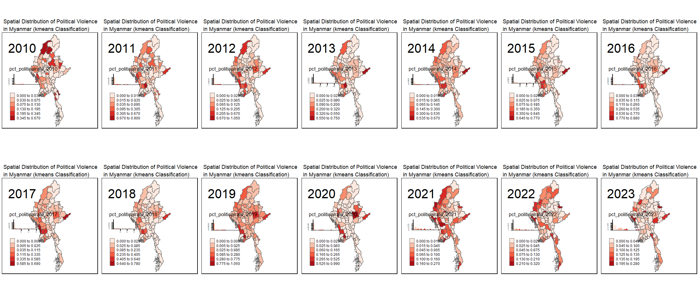
Spatial Distribution of Violence Against Civilians (2010 to 2023)
Show code
cv10 <- tm_shape(mapping_rates) +
tm_fill("pct_civilianrate_2010",
n = 6,
style = "kmeans",
palette = "Reds",
legend.hist = TRUE,
legend.is.portrait = TRUE,
legend.hist.z = 0.1) +
tm_borders(lwd = 0.1,
alpha = 1) +
tm_layout(main.title = "Spatial Distribution of Violence against Civilians \nin Myanmar (kmeans Classification)",
title = "2010",
main.title.size = 0.55,
legend.height = 0.60,
legend.width = 5.0,
legend.outside = FALSE,
legend.position = c("left", "bottom"))
cv11 <- tm_shape(mapping_rates) +
tm_fill("pct_civilianrate_2011",
n = 6,
style = "kmeans",
palette = "Reds",
legend.hist = TRUE,
legend.is.portrait = TRUE,
legend.hist.z = 0.1) +
tm_borders(lwd = 0.1,
alpha = 1) +
tm_layout(main.title = "Spatial Distribution of Violence against Civilians \nin Myanmar (kmeans Classification)",
title = "2011",
main.title.size = 0.55,
legend.height = 0.60,
legend.width = 5.0,
legend.outside = FALSE,
legend.position = c("left", "bottom"))
cv12 <- tm_shape(mapping_rates) +
tm_fill("pct_civilianrate_2012",
n = 6,
style = "kmeans",
palette = "Reds",
legend.hist = TRUE,
legend.is.portrait = TRUE,
legend.hist.z = 0.1) +
tm_borders(lwd = 0.1,
alpha = 1) +
tm_layout(main.title = "Spatial Distribution of Violence against Civilians \nin Myanmar (kmeans Classification)",
title = "2012",
main.title.size = 0.55,
legend.height = 0.60,
legend.width = 5.0,
legend.outside = FALSE,
legend.position = c("left", "bottom"))
cv13 <- tm_shape(mapping_rates) +
tm_fill("pct_civilianrate_2013",
n = 6,
style = "kmeans",
palette = "Reds",
legend.hist = TRUE,
legend.is.portrait = TRUE,
legend.hist.z = 0.1) +
tm_borders(lwd = 0.1,
alpha = 1) +
tm_layout(main.title = "Spatial Distribution of Violence against Civilians \nin Myanmar (kmeans Classification)",
title = "2013",
main.title.size = 0.55,
legend.height = 0.60,
legend.width = 5.0,
legend.outside = FALSE,
legend.position = c("left", "bottom"))
cv14 <- tm_shape(mapping_rates) +
tm_fill("pct_civilianrate_2014",
n = 6,
style = "kmeans",
palette = "Reds",
legend.hist = TRUE,
legend.is.portrait = TRUE,
legend.hist.z = 0.1) +
tm_borders(lwd = 0.1,
alpha = 1) +
tm_layout(main.title = "Spatial Distribution of Violence against Civilians \nin Myanmar (kmeans Classification)",
title = "2014",
main.title.size = 0.55,
legend.height = 0.60,
legend.width = 5.0,
legend.outside = FALSE,
legend.position = c("left", "bottom"))
cv15 <- tm_shape(mapping_rates) +
tm_fill("pct_civilianrate_2015",
n = 6,
style = "kmeans",
palette = "Reds",
legend.hist = TRUE,
legend.is.portrait = TRUE,
legend.hist.z = 0.1) +
tm_borders(lwd = 0.1,
alpha = 1) +
tm_layout(main.title = "Spatial Distribution of Violence against Civilians \nin Myanmar (kmeans Classification)",
title = "2015",
main.title.size = 0.55,
legend.height = 0.60,
legend.width = 5.0,
legend.outside = FALSE,
legend.position = c("left", "bottom"))
cv16 <- tm_shape(mapping_rates) +
tm_fill("pct_civilianrate_2016",
n = 6,
style = "kmeans",
palette = "Reds",
legend.hist = TRUE,
legend.is.portrait = TRUE,
legend.hist.z = 0.1) +
tm_borders(lwd = 0.1,
alpha = 1) +
tm_layout(main.title = "Spatial Distribution of Violence against Civilians \nin Myanmar (kmeans Classification)",
title = "2016",
main.title.size = 0.55,
legend.height = 0.60,
legend.width = 5.0,
legend.outside = FALSE,
legend.position = c("left", "bottom"))
cv17 <- tm_shape(mapping_rates) +
tm_fill("pct_civilianrate_2017",
n = 6,
style = "kmeans",
palette = "Reds",
legend.hist = TRUE,
legend.is.portrait = TRUE,
legend.hist.z = 0.1) +
tm_borders(lwd = 0.1,
alpha = 1) +
tm_layout(main.title = "Spatial Distribution of Violence against Civilians \nin Myanmar (kmeans Classification)",
title = "2017",
main.title.size = 0.55,
legend.height = 0.60,
legend.width = 5.0,
legend.outside = FALSE,
legend.position = c("left", "bottom"))
cv18 <- tm_shape(mapping_rates) +
tm_fill("pct_civilianrate_2018",
n = 6,
style = "kmeans",
palette = "Reds",
legend.hist = TRUE,
legend.is.portrait = TRUE,
legend.hist.z = 0.1) +
tm_borders(lwd = 0.1,
alpha = 1) +
tm_layout(main.title = "Spatial Distribution of Violence against Civilians \nin Myanmar (kmeans Classification)",
title = "2018",
main.title.size = 0.55,
legend.height = 0.60,
legend.width = 5.0,
legend.outside = FALSE,
legend.position = c("left", "bottom"))
cv19 <- tm_shape(mapping_rates) +
tm_fill("pct_civilianrate_2019",
n = 6,
style = "kmeans",
palette = "Reds",
legend.hist = TRUE,
legend.is.portrait = TRUE,
legend.hist.z = 0.1) +
tm_borders(lwd = 0.1,
alpha = 1) +
tm_layout(main.title = "Spatial Distribution of Violence against Civilians \nin Myanmar (kmeans Classification)",
title = "2019",
main.title.size = 0.55,
legend.height = 0.60,
legend.width = 5.0,
legend.outside = FALSE,
legend.position = c("left", "bottom"))
cv20 <- tm_shape(mapping_rates) +
tm_fill("pct_civilianrate_2020",
n = 6,
style = "kmeans",
palette = "Reds",
legend.hist = TRUE,
legend.is.portrait = TRUE,
legend.hist.z = 0.1) +
tm_borders(lwd = 0.1,
alpha = 1) +
tm_layout(main.title = "Spatial Distribution of Violence against Civilians \nin Myanmar (kmeans Classification)",
title = "2020",
main.title.size = 0.55,
legend.height = 0.60,
legend.width = 5.0,
legend.outside = FALSE,
legend.position = c("left", "bottom"))
cv21 <- tm_shape(mapping_rates) +
tm_fill("pct_civilianrate_2021",
n = 6,
style = "kmeans",
palette = "Reds",
legend.hist = TRUE,
legend.is.portrait = TRUE,
legend.hist.z = 0.1) +
tm_borders(lwd = 0.1,
alpha = 1) +
tm_layout(main.title = "Spatial Distribution of Violence against Civilians \nin Myanmar (kmeans Classification)",
title = "2021",
main.title.size = 0.55,
legend.height = 0.60,
legend.width = 5.0,
legend.outside = FALSE,
legend.position = c("left", "bottom"))
cv22 <- tm_shape(mapping_rates) +
tm_fill("pct_civilianrate_2022",
n = 6,
style = "kmeans",
palette = "Reds",
legend.hist = TRUE,
legend.is.portrait = TRUE,
legend.hist.z = 0.1) +
tm_borders(lwd = 0.1,
alpha = 1) +
tm_layout(main.title = "Spatial Distribution of Violence against Civilians \nin Myanmar (kmeans Classification)",
title = "2022",
main.title.size = 0.55,
legend.height = 0.60,
legend.width = 5.0,
legend.outside = FALSE,
legend.position = c("left", "bottom"))
cv23 <- tm_shape(mapping_rates) +
tm_fill("pct_civilianrate_2023",
n = 6,
style = "kmeans",
palette = "Reds",
legend.hist = TRUE,
legend.is.portrait = TRUE,
legend.hist.z = 0.1) +
tm_borders(lwd = 0.1,
alpha = 1) +
tm_layout(main.title = "Spatial Distribution of Violence against Civilians \nin Myanmar (kmeans Classification)",
title = "2023",
main.title.size = 0.55,
legend.height = 0.60,
legend.width = 5.0,
legend.outside = FALSE,
legend.position = c("left", "bottom"))Show code
tmap_arrange(cv10, cv11, cv12, cv13, cv14, cv15, cv16,
cv17, cv18, cv19, cv20, cv21, cv22, cv23,
asp = 1,
ncol=7, nrow=2)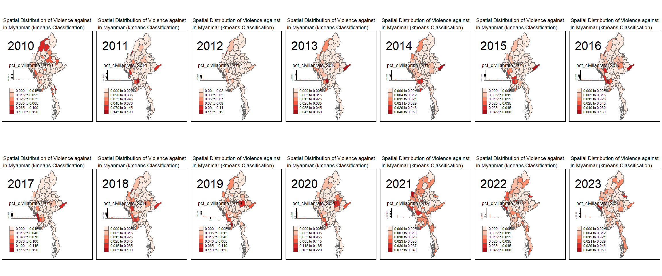
Spatial Distribution of Fatalities (2010 to 2023)
Show code
f10 <- tm_shape(mapping_rates) +
tm_fill("pct_fata_2010",
n = 6,
style = "kmeans",
palette = "Reds",
legend.hist = TRUE,
legend.is.portrait = TRUE,
legend.hist.z = 0.1) +
tm_borders(lwd = 0.1,
alpha = 1) +
tm_layout(main.title = "Spatial Distribution of Fatalities \nin Myanmar (kmeans Classification)",
title = "2010",
main.title.size = 0.55,
legend.height = 0.60,
legend.width = 5.0,
legend.outside = FALSE,
legend.position = c("left", "bottom"))
f11 <- tm_shape(mapping_rates) +
tm_fill("pct_fata_2011",
n = 6,
style = "kmeans",
palette = "Reds",
legend.hist = TRUE,
legend.is.portrait = TRUE,
legend.hist.z = 0.1) +
tm_borders(lwd = 0.1,
alpha = 1) +
tm_layout(main.title = "Spatial Distribution of Fatalities \nin Myanmar (kmeans Classification)",
title = "2011",
main.title.size = 0.55,
legend.height = 0.60,
legend.width = 5.0,
legend.outside = FALSE,
legend.position = c("left", "bottom"))
f12 <- tm_shape(mapping_rates) +
tm_fill("pct_fata_2012",
n = 6,
style = "kmeans",
palette = "Reds",
legend.hist = TRUE,
legend.is.portrait = TRUE,
legend.hist.z = 0.1) +
tm_borders(lwd = 0.1,
alpha = 1) +
tm_layout(main.title = "Spatial Distribution of Fatalities \nin Myanmar (kmeans Classification)",
title = "2012",
main.title.size = 0.55,
legend.height = 0.60,
legend.width = 5.0,
legend.outside = FALSE,
legend.position = c("left", "bottom"))
f13 <- tm_shape(mapping_rates) +
tm_fill("pct_fata_2013",
n = 6,
style = "kmeans",
palette = "Reds",
legend.hist = TRUE,
legend.is.portrait = TRUE,
legend.hist.z = 0.1) +
tm_borders(lwd = 0.1,
alpha = 1) +
tm_layout(main.title = "Spatial Distribution of Fatalities \nin Myanmar (kmeans Classification)",
title = "2013",
main.title.size = 0.55,
legend.height = 0.60,
legend.width = 5.0,
legend.outside = FALSE,
legend.position = c("left", "bottom"))
f14 <- tm_shape(mapping_rates) +
tm_fill("pct_fata_2014",
n = 6,
style = "kmeans",
palette = "Reds",
legend.hist = TRUE,
legend.is.portrait = TRUE,
legend.hist.z = 0.1) +
tm_borders(lwd = 0.1,
alpha = 1) +
tm_layout(main.title = "Spatial Distribution of Fatalities \nin Myanmar (kmeans Classification)",
title = "2014",
main.title.size = 0.55,
legend.height = 0.60,
legend.width = 5.0,
legend.outside = FALSE,
legend.position = c("left", "bottom"))
f15 <- tm_shape(mapping_rates) +
tm_fill("pct_fata_2015",
n = 6,
style = "kmeans",
palette = "Reds",
legend.hist = TRUE,
legend.is.portrait = TRUE,
legend.hist.z = 0.1) +
tm_borders(lwd = 0.1,
alpha = 1) +
tm_layout(main.title = "Spatial Distribution of Fatalities \nin Myanmar (kmeans Classification)",
title = "2015",
main.title.size = 0.55,
legend.height = 0.60,
legend.width = 5.0,
legend.outside = FALSE,
legend.position = c("left", "bottom"))
f16 <- tm_shape(mapping_rates) +
tm_fill("pct_fata_2016",
n = 6,
style = "kmeans",
palette = "Reds",
legend.hist = TRUE,
legend.is.portrait = TRUE,
legend.hist.z = 0.1) +
tm_borders(lwd = 0.1,
alpha = 1) +
tm_layout(main.title = "Spatial Distribution of Fatalities \nin Myanmar (kmeans Classification)",
title = "2016",
main.title.size = 0.55,
legend.height = 0.60,
legend.width = 5.0,
legend.outside = FALSE,
legend.position = c("left", "bottom"))
f17 <- tm_shape(mapping_rates) +
tm_fill("pct_fata_2017",
n = 6,
style = "kmeans",
palette = "Reds",
legend.hist = TRUE,
legend.is.portrait = TRUE,
legend.hist.z = 0.1) +
tm_borders(lwd = 0.1,
alpha = 1) +
tm_layout(main.title = "Spatial Distribution of Fatalities \nin Myanmar (kmeans Classification)",
title = "2017",
main.title.size = 0.55,
legend.height = 0.60,
legend.width = 5.0,
legend.outside = FALSE,
legend.position = c("left", "bottom"))
f18 <- tm_shape(mapping_rates) +
tm_fill("pct_fata_2018",
n = 6,
style = "kmeans",
palette = "Reds",
legend.hist = TRUE,
legend.is.portrait = TRUE,
legend.hist.z = 0.1) +
tm_borders(lwd = 0.1,
alpha = 1) +
tm_layout(main.title = "Spatial Distribution of Fatalities \nin Myanmar (kmeans Classification)",
title = "2018",
main.title.size = 0.55,
legend.height = 0.60,
legend.width = 5.0,
legend.outside = FALSE,
legend.position = c("left", "bottom"))
f19 <- tm_shape(mapping_rates) +
tm_fill("pct_fata_2019",
n = 6,
style = "kmeans",
palette = "Reds",
legend.hist = TRUE,
legend.is.portrait = TRUE,
legend.hist.z = 0.1) +
tm_borders(lwd = 0.1,
alpha = 1) +
tm_layout(main.title = "Spatial Distribution of Fatalities \nin Myanmar (kmeans Classification)",
title = "2019",
main.title.size = 0.55,
legend.height = 0.60,
legend.width = 5.0,
legend.outside = FALSE,
legend.position = c("left", "bottom"))
f20 <- tm_shape(mapping_rates) +
tm_fill("pct_fata_2020",
n = 6,
style = "kmeans",
palette = "Reds",
legend.hist = TRUE,
legend.is.portrait = TRUE,
legend.hist.z = 0.1) +
tm_borders(lwd = 0.1,
alpha = 1) +
tm_layout(main.title = "Spatial Distribution of Fatalities \nin Myanmar (kmeans Classification)",
title = "2020",
main.title.size = 0.55,
legend.height = 0.60,
legend.width = 5.0,
legend.outside = FALSE,
legend.position = c("left", "bottom"))
f21 <- tm_shape(mapping_rates) +
tm_fill("pct_fata_2021",
n = 6,
style = "kmeans",
palette = "Reds",
legend.hist = TRUE,
legend.is.portrait = TRUE,
legend.hist.z = 0.1) +
tm_borders(lwd = 0.1,
alpha = 1) +
tm_layout(main.title = "Spatial Distribution of Fatalities \nin Myanmar (kmeans Classification)",
title = "2021",
main.title.size = 0.55,
legend.height = 0.60,
legend.width = 5.0,
legend.outside = FALSE,
legend.position = c("left", "bottom"))
f22 <- tm_shape(mapping_rates) +
tm_fill("pct_fata_2022",
n = 6,
style = "kmeans",
palette = "Reds",
legend.hist = TRUE,
legend.is.portrait = TRUE,
legend.hist.z = 0.1) +
tm_borders(lwd = 0.1,
alpha = 1) +
tm_layout(main.title = "Spatial Distribution of Fatalities \nin Myanmar (kmeans Classification)",
title = "2022",
main.title.size = 0.55,
legend.height = 0.60,
legend.width = 5.0,
legend.outside = FALSE,
legend.position = c("left", "bottom"))
f23 <- tm_shape(mapping_rates) +
tm_fill("pct_fata_2023",
n = 6,
style = "kmeans",
palette = "Reds",
legend.hist = TRUE,
legend.is.portrait = TRUE,
legend.hist.z = 0.1) +
tm_borders(lwd = 0.1,
alpha = 1) +
tm_layout(main.title = "Spatial Distribution of Fatalities \nin Myanmar (kmeans Classification)",
title = "2023",
main.title.size = 0.55,
legend.height = 0.60,
legend.width = 5.0,
legend.outside = FALSE,
legend.position = c("left", "bottom"))Show code
tmap_arrange(f10, f11, f12, f13, f14, f15, f16,
f17, f18, f19, f20, f21, f22, f23,
asp = 1,
ncol=7, nrow=2)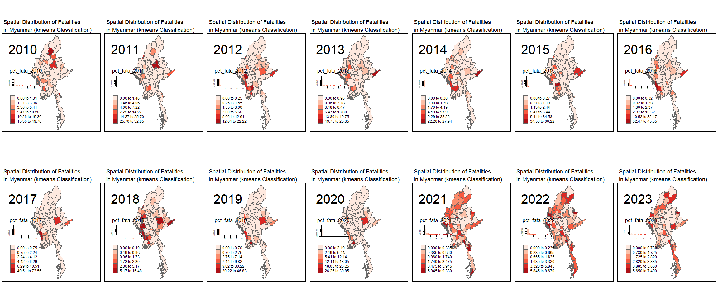
Interactive Choropleth Map (Spatial Distribution)
An example below is an interactive spatial map, which uses tmap_leaflet() a leaflet widget from tmap object. This code chunk will be used to plot interactive maps for spatial statistical distribution, spatial area density and spatial distribution.
Show code
tmap_obj <- tm_shape(mapping_rates) +
tm_fill("total_inci",
n = 6,
style = "kmeans",
palette = "Reds",
legend.hist = TRUE,
legend.is.portrait = TRUE,
legend.hist.z = 0.1) +
tm_borders(lwd = 0.1, alpha = 1) +
tm_layout(main.title = "Distribution of Armed Conflict Incidents in Myanmar \nKmeans classification",
title = "(2010-2023)",
main.title.size = 1,
legend.height = 0.60,
legend.width = 5.0,
legend.outside = FALSE,
legend.position = c("left", "bottom"))
leaflet_map <- tmap_leaflet(tmap_obj) %>%
addTiles('https://basemaps.cartocdn.com/light_all/{z}/{x}/{y}.png') %>%
addPolygons(data = mapping_rates,
label = ~paste("Custom Tooltip Content: ",
mapping_rates$total_inci, "\n",
mapping_rates$total_fata))
leaflet_map3.4 Spatial Points
To visualise the spatial points (armed conflict events) based on their geographical coordinates. longitude and latitude are used to plot the point symbol map.
Interactive Point Symbol Map (Spatial Points)
Leaflet() is used to plot the interactive map and addCircles() is used to plot the individual armed conflict incidents.
Show code
cof <- colorFactor(c("#ff7e8a", "#394938", "#ffa500",
"#0092ff", "#741b47", "#60dcb5"),
domain=c("Battles", "Explosions/ Remote violence",
"Protests", "Riots",
"Strategic developments",
"Violence against civilians"))
incident_pts <- final %>%
filter(fatalities > 0)
psmap <- leaflet() %>%
addTiles('https://basemaps.cartocdn.com/light_all/{z}/{x}/{y}.png') %>%
setView(100, 20, zoom = 5) %>%
addCircles(data=incident_pts, lat= ~latitude, lng = ~longitude,
color = ~cof(event_type),
fillColor = "black",
popup = paste( "<strong>", incident_pts$event_date, "</strong>",
"<br><strong>Country: </strong>",
incident_pts$country,
"<br><strong>Sub-national Admin Region: </strong>",
incident_pts$admin1, "/",
incident_pts$admin2, "/",
incident_pts$admin3,
"<br><strong>Event type: </strong>",
incident_pts$event_type,
"<br><strong>Sub-event type: </strong>",
incident_pts$sub_event_type,
"<br><strong>Summary: </strong>",
incident_pts$notes,
"<br><strong>Total Fatalities: </strong>",
incident_pts$fatalities)) %>%
addLegend("bottomright",
colors = c("#ff7e8a", "#394938", "#ffa500",
"#0092ff", "#741b47", "#60dcb5"),
labels = c("Battles", "Explosions/ Remote violence", "Protests",
"Riots", "Strategic developments",
"Violence against civilians"), title="Event Type")
psmap3.5 Spatial Concentration/ Intensity
To visualise the spatial concentration/ intensity of armed conflict events, longitude and latitude are used to plot the heatmap map.
leaflet() is used to plot the interactive map and addHeatmap() is used to plot the intensity based on the settings of max, radius and blur values.
Show code
incident_pts <- final %>%
filter(fatalities > 0)
# create fatalities hotspot intensity
hotmap_fata <- leaflet() %>%
addTiles('https://basemaps.cartocdn.com/light_all/{z}/{x}/{y}.png') %>%
setView(100, 20, zoom = 5) %>%
addHeatmap(data=incident_pts, lng = ~longitude, lat = ~latitude,
intensity = ~total_fata, max = 100, radius = 10, blur = 10)
incident_pts <- final %>%
filter(fatalities > 0)
# create armed conflict incidents hotspot intensity
hotmap_inci <- leaflet() %>%
addTiles('https://basemaps.cartocdn.com/light_all/{z}/{x}/{y}.png') %>%
setView(100, 20, zoom = 5) %>%
addHeatmap(data=incident_pts, lng = ~longitude, lat = ~latitude,
intensity = ~total_inci, max = 100, radius = 10, blur = 10) %>%
addPopups(data = incident_pts, lng = ~longitude, lat = ~latitude,
popup = ~paste("<strong>Date: </strong>", event_date,
"<br><strong>Country: </strong>", country))
# latticeview(hotmap_fata, hotmap_inci)
hotmap_fataThe code chunk below turns off plot mode.
# switch tmap off
tmap_mode("plot")4 Prototype: Exploratory
Prototype: Exploratory can be found via link here.
This segment has been separated on a standalone web page due to Quarto rendering capacity.