Hands-on Exercise 5 - Part 5

Treemap Visualisation with R

Note: Last modified to include author’s details.

1. Getting Started

Plot static treemap using treemap package.

Design interactive treemap using d3treeR package.

1.1 Install and launch R packages

For the purpose of this exercise, the following R packages will be used.

For Static Treemap (Section 2.1 & 2.2)

pacman::p_load(treemap, treemapify, tidyverse)

For Interactive Treemap (Section 2.3)

1. First-time users will have to install additional package from github with the code chunk below. Otherwise, proceed to step 3 to launch d3treeR package.

install.packages("devtools")

2. Load devtools library and install package found in github with the code chunk below.

library(devtools)
install_github("timelyportfolio/d3treeR", force = TRUE)

3. Launch d3treeR package with code chunk below.

library(d3treeR)

1.2 Import the data

This exercise used the REALIS2018.csv data from Urban Redevelopment Authority (URA) - REALIS portal. This dataset provides information of private property transaction records in 2018.

Code

realis2018 <- read_csv("data/realis2018.csv")

1.3 Overview of the data

Show code

summary(realis2018)

 Project Name         Address           No. of Units   Area (sqm)    
 Length:23205       Length:23205       Min.   :1     Min.   :  24.0  
 Class :character   Class :character   1st Qu.:1     1st Qu.:  67.0  
 Mode  :character   Mode  :character   Median :1     Median :  98.0  
                                       Mean   :1     Mean   : 118.2  
                                       3rd Qu.:1     3rd Qu.: 127.0  
                                       Max.   :1     Max.   :4836.0  
 Type of Area       Transacted Price ($) Nett Price($)      Unit Price ($ psm)
 Length:23205       Min.   :    40000    Length:23205       Min.   :  355     
 Class :character   1st Qu.:   950000    Class :character   1st Qu.:11231     
 Mode  :character   Median :  1280000    Mode  :character   Median :14621     
                    Mean   :  1734099                       Mean   :15246     
                    3rd Qu.:  1858000                       3rd Qu.:18075     
                    Max.   :100000000                       Max.   :54363     
 Unit Price ($ psf)  Sale Date         Property Type         Tenure         
 Min.   :  33       Length:23205       Length:23205       Length:23205      
 1st Qu.:1043       Class :character   Class :character   Class :character  
 Median :1358       Mode  :character   Mode  :character   Mode  :character  
 Mean   :1416                                                               
 3rd Qu.:1679                                                               
 Max.   :5050                                                               
 Completion Date    Type of Sale       Purchaser Address Indicator
 Length:23205       Length:23205       Length:23205               
 Class :character   Class :character   Class :character           
 Mode  :character   Mode  :character   Mode  :character           
                                                                  
                                                                  
                                                                  
 Postal District Postal Sector    Postal Code     Planning Region   
 Min.   : 1.00   Min.   : 1.00   Min.   : 18965   Length:23205      
 1st Qu.:10.00   1st Qu.:26.00   1st Qu.:267952   Class :character  
 Median :15.00   Median :45.00   Median :456068   Mode  :character  
 Mean   :14.96   Mean   :42.66   Mean   :434269                     
 3rd Qu.:19.00   3rd Qu.:54.00   3rd Qu.:548461                     
 Max.   :28.00   Max.   :82.00   Max.   :829750                     
 Planning Area     
 Length:23205      
 Class :character  
 Mode  :character  
                   
                   
                   

1.4 Data Wrangling & Manipulation

Data Frame realis2018

• Highly disaggregated and not appropriate to be used to plot a treemap

• Need to manipulate and prepare for another data frame for treemap visualisation:

  • group transaction records by Project Name, Planning Region, Planning Area, Property Type and Type of Sale, and

  • compute Total Unit Sold, Total Area, Median Unit Price and Median Transacted Price by applying appropriate summary statistics on No. of Units, Area (sqm), Unit Price ($ psm) and Transacted Price ($) respectively.

Two key verbs of dplyr package, namely: group_by() and summarize() will be used to perform these steps.

group_by() breaks down a data.frame into specified groups of rows. When you then apply the verbs above on the resulting object they’ll be automatically applied “by group”.

Grouping affects the verbs as follows:

• grouped select() is the same as ungrouped select(), except that grouping variables are always retained.

• grouped arrange() is the same as ungrouped; unless you set .by_group = TRUE, in which case it orders first by the grouping variables.

• mutate() and filter() are most useful in conjunction with window functions (like rank(), or min(x) == x). They are described in detail in vignette(“window-functions”).

• sample_n() and sample_frac() sample the specified number/fraction of rows in each group.

• summarise() computes the summary for each group.

Show code

realis2018_grouped <- group_by(realis2018, `Project Name`,
                               `Planning Region`, `Planning Area`, 
                               `Property Type`, `Type of Sale`)
realis2018_summarised <- summarise(realis2018_grouped, 
                          `Total Unit Sold` = sum(`No. of Units`, na.rm = TRUE),
                          `Total Area` = sum(`Area (sqm)`, na.rm = TRUE),
                          `Median Unit Price ($ psm)` = median(`Unit Price ($ psm)`, na.rm = TRUE), 
                          `Median Transacted Price` = median(`Transacted Price ($)`, na.rm = TRUE))

Learning Points

• group_by() is used together with summarise() to derive the summarised data.frame.

• Aggregation functions such as sum() and meadian() obey the usual rule of missing values: if there’s any missing value in the input, the output will be a missing value. The argument na.rm = TRUE removes the missing values prior to computation.

• The code chunk above is not very efficient given the need to name each intermediate data.frame, e.g. realis2018_grouped and realis2018_summarised (though not necessary).

Group summaries with pipe

The code chunk below shows a more efficient way to tackle the same processes by using the pipe, %>%:

Show code

realis2018_summarised <- realis2018 %>% 
  group_by(`Project Name`,`Planning Region`, 
           `Planning Area`, `Property Type`, 
           `Type of Sale`) %>%
  summarise(`Total Unit Sold` = sum(`No. of Units`, na.rm = TRUE), 
            `Total Area` = sum(`Area (sqm)`, na.rm = TRUE),
            `Median Unit Price ($ psm)` = median(`Unit Price ($ psm)`, na.rm = TRUE),
            `Median Transacted Price` = median(`Transacted Price ($)`, na.rm = TRUE))

2. Designing Treemap with treemap package

2.1 Designing Static Treemap

treemap package is a R package specially designed to offer great flexibility in drawing treemaps. The core function, namely: treemap() offers at least 43 arguments.

2.1.1 Using basic arugments

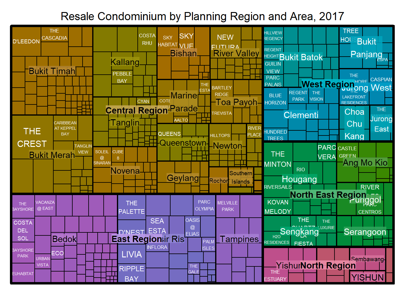
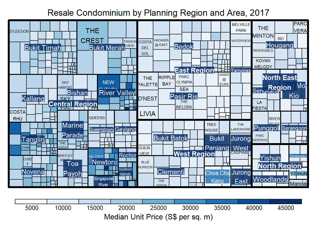
treemap() of Treemap package is used to plot a treemap showing the distribution of median unit prices and total unit sold of resale condominium by geographic hierarchy in 2017.

Select records that belong to resale condominium property type.

Show code

realis2018_selected <- realis2018_summarised %>%
  filter(`Property Type` == "Condominium", `Type of Sale` == "Resale")

The code chunk below designed a treemap by using three core arguments of treemap(), namely: index, vSize and vColor.

Show code

treemap(realis2018_selected,
        index=c("Planning Region", "Planning Area", "Project Name"),
        vSize="Total Unit Sold",
        vColor="Median Unit Price ($ psm)",
        title="Resale Condominium by Planning Region and Area, 2017",
        title.legend = "Median Unit Price (S$ per sq. m)"
        )

Learning Points

• index

  • The index vector must consist of at least two column names or else no hierarchy treemap will be plotted.

  • If multiple column names are provided, such as the code chunk above, the first name is the highest aggregation level, the second name the second highest aggregation level, and so on.

• vSize

  • The column must not contain negative values. This is because the vaues will be used to map the sizes of the rectangles of the treemaps.

• vColor

  • The treemap above was wrongly coloured. For a correctly designed treemap, the colours of the rectagles should be in different intensity showing (in median unit prices).

  • vColor is used in combination with the argument type to determines the colours of the rectangles. Without defining type, like the code chunk above, treemap() assumes type = index, (the hierarchy of planning areas).

2.1.2 Working with vColor and type arguments

Two arguments that determine the mapping to color palettes: mapping and palette.

The only difference between “value” and “manual” is the default value for mapping.

The “value” treemap considers palette to be a diverging color palette (e.g ColorBrewer’s “RdYlBu”), and maps it in such a way that 0 corresponds to the middle color (typically white or yellow), -max(abs(values)) to the left-end color, and max(abs(values)) to the right-end color.

The “manual” treemap simply maps min(values) to the left-end color, max(values) to the right-end color, and mean(range(values)) to the middle color.

type = “value”

In the code chunk below, type argument is define as value.

Show code

treemap(realis2018_selected,
        index=c("Planning Region", "Planning Area", "Project Name"),
        vSize="Total Unit Sold",
        vColor="Median Unit Price ($ psm)",
        type = "value",
        title="Resale Condominium by Planning Region and Area, 2017",
        title.legend = "Median Unit Price (S$ per sq. m)"
        )

Learning Points

• The rectangles are coloured with different intensity of green, reflecting their respective median unit prices.

• The legend reveals that the values are binned into ten bins, i.e. 0-5000, 5000-10000, etc. with an equal interval of 5000.

type = “value”, palette=“”

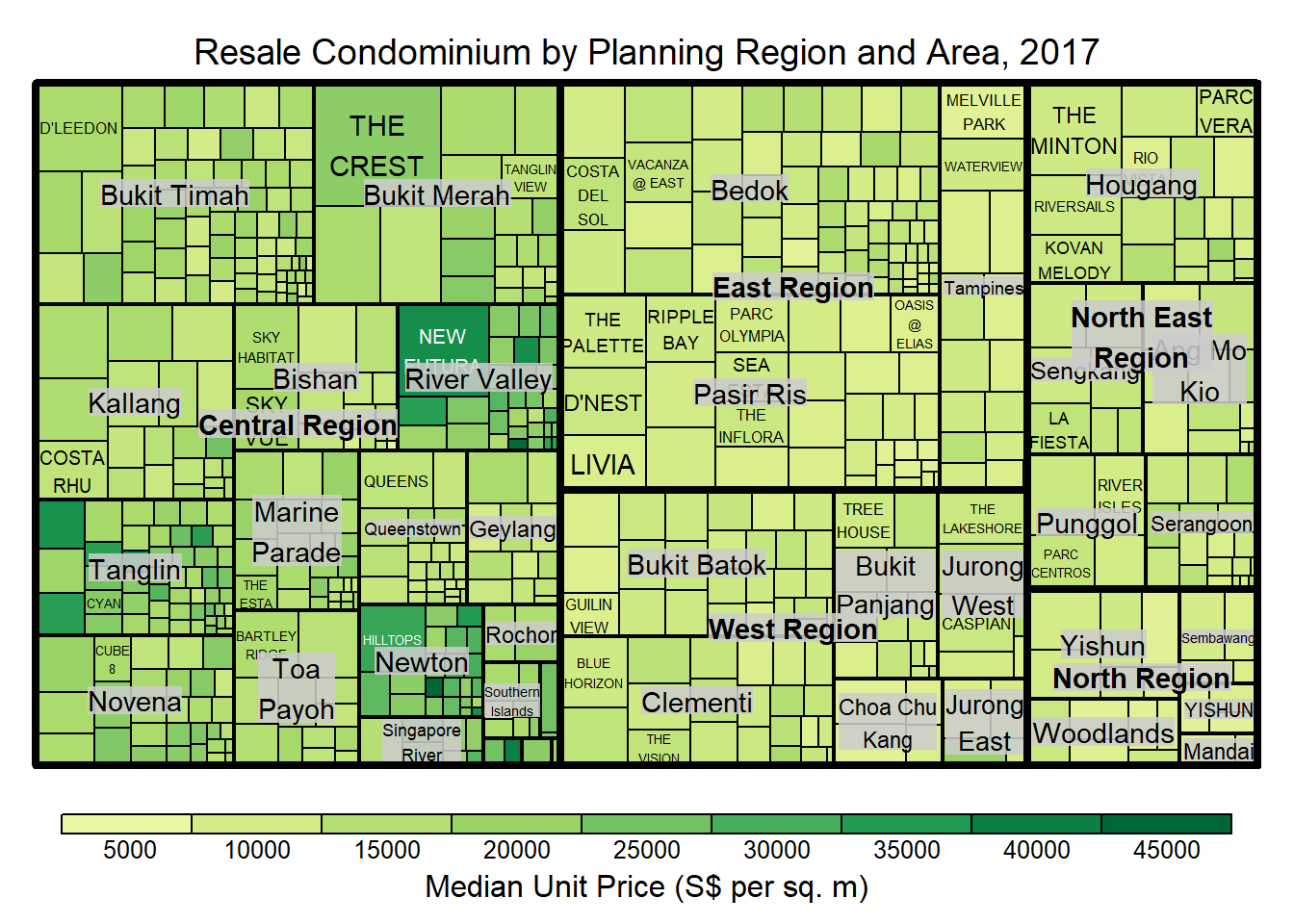
In the code chunk below:

• type argument is define as value

• palette = “RdYlBu”

Show code

treemap(realis2018_selected,
        index=c("Planning Region", "Planning Area", "Project Name"),
        vSize="Total Unit Sold",
        vColor="Median Unit Price ($ psm)",
        type="value",
        palette="RdYlBu", 
        title="Resale Condominium by Planning Region and Area, 2017",
        title.legend = "Median Unit Price (S$ per sq. m)"
        )

Learning Points

• Note that the colour palette “RdYlBu” is used but there are no red rectangles in the treemap above. This is because all the median unit prices are positive values.

  • Legend only reveals range between 5000 to 45000 because the range argument is by default c(min(values, max(values)).

type = “manual” [wrong palette]

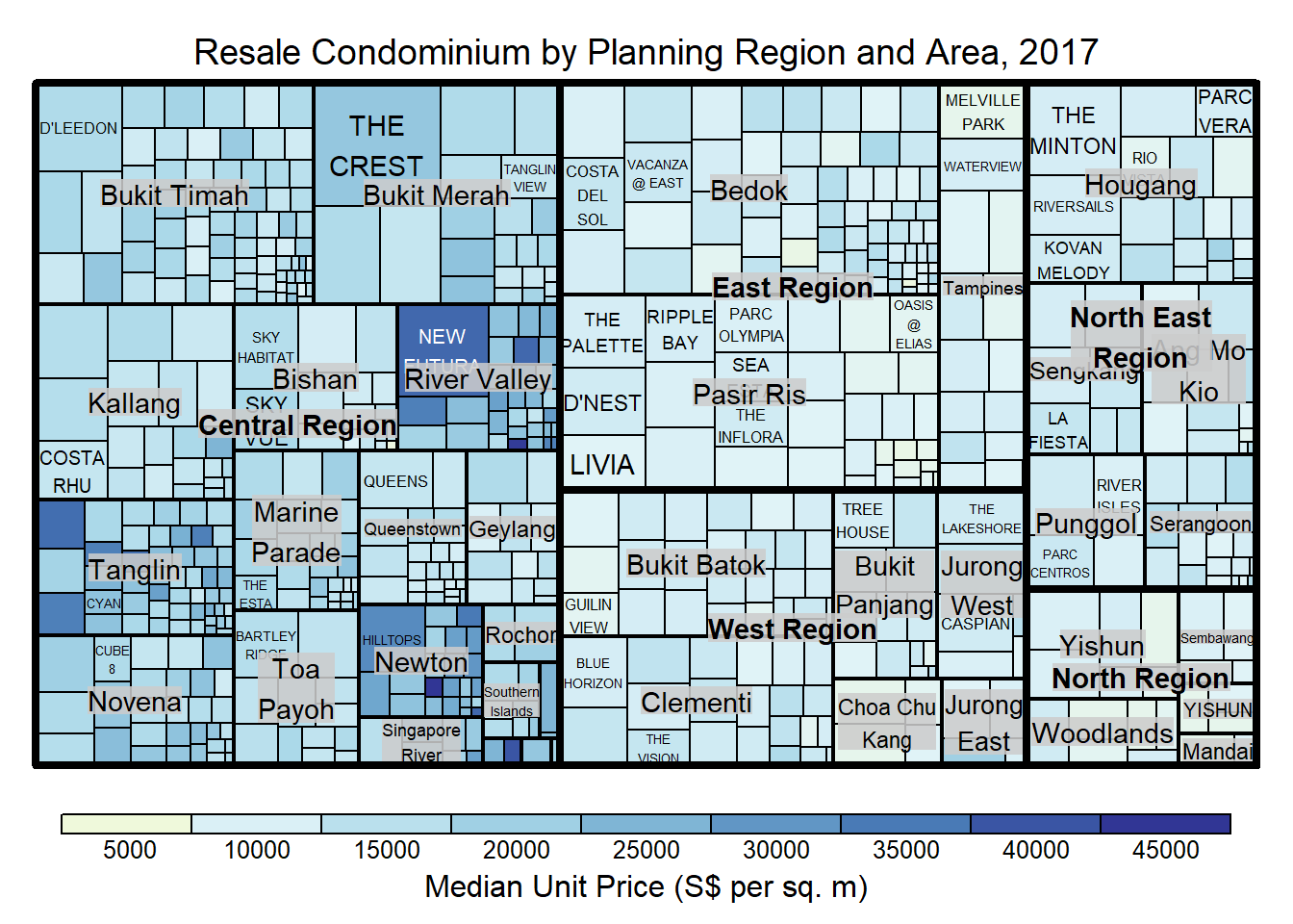
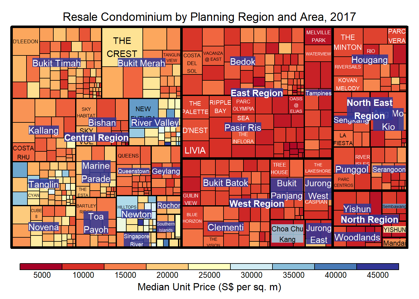
The “manual” type does not interpret the values as the “value” type does. Instead, the value range is mapped linearly to the colour palette.

Show code

treemap(realis2018_selected,
        index=c("Planning Region", "Planning Area", "Project Name"),
        vSize="Total Unit Sold",
        vColor="Median Unit Price ($ psm)",
        type="manual",
        palette="RdYlBu", 
        title="Resale Condominium by Planning Region and Area, 2017",
        title.legend = "Median Unit Price (S$ per sq. m)"
        )

Learning Points

• colour scheme used is very confusing because of mapping = (min(values), mean(range(values)), max(values)).

• It is not wise to use diverging colour palette such as RdYlBu if the values are all positive or negative

type = “manual” [correct palette]

Show code

treemap(realis2018_selected,
        index=c("Planning Region", "Planning Area", "Project Name"),
        vSize="Total Unit Sold",
        vColor="Median Unit Price ($ psm)",
        type="manual",
        palette="Blues", 
        title="Resale Condominium by Planning Region and Area, 2017",
        title.legend = "Median Unit Price (S$ per sq. m)"
        )

2.1.2 Working with treemap layout algorithm argument

Treemap Layout

treemap() supports two popular treemap layouts, namely: “squarified” and “pivotSize”. The default is “pivotSize”.

• squarified treemap algorithm (Bruls et al., 2000) produces good aspect ratios, but ignores the sorting order of the rectangles (sortID).

• ordered treemap, pivot-by-size, algorithm (Bederson et al., 2002) takes the sorting order (sortID) into account while aspect ratios are still acceptable.

  squarified treemap

  Set algorithm = "squarified" for squarified treemap

  Show code

  treemap(realis2018_selected,
          index=c("Planning Region", "Planning Area", "Project Name"),
          vSize="Total Unit Sold",
          vColor="Median Unit Price ($ psm)",
          type="manual",
          palette="Blues", 
          algorithm = "squarified",
          title="Resale Condominium by Planning Region and Area, 2017",
          title.legend = "Median Unit Price (S$ per sq. m)"
          )

  

  ordered treemap

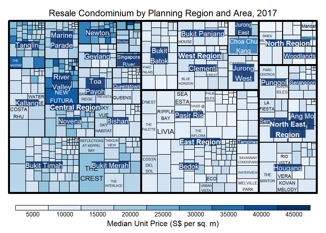
  Set algorithm = "pivotSize" for ordered treemap.

  Use sortID argument to determine order in which the rectangles are placed from top left to bottom right.

  Show code

  treemap(realis2018_selected,
          index=c("Planning Region", "Planning Area", "Project Name"),
          vSize="Total Unit Sold",
          vColor="Median Unit Price ($ psm)",
          type="manual",
          palette="Blues", 
          algorithm = "pivotSize",
          sortID = "Median Transacted Price",
          title="Resale Condominium by Planning Region and Area, 2017",
          title.legend = "Median Unit Price (S$ per sq. m)"
          )

  

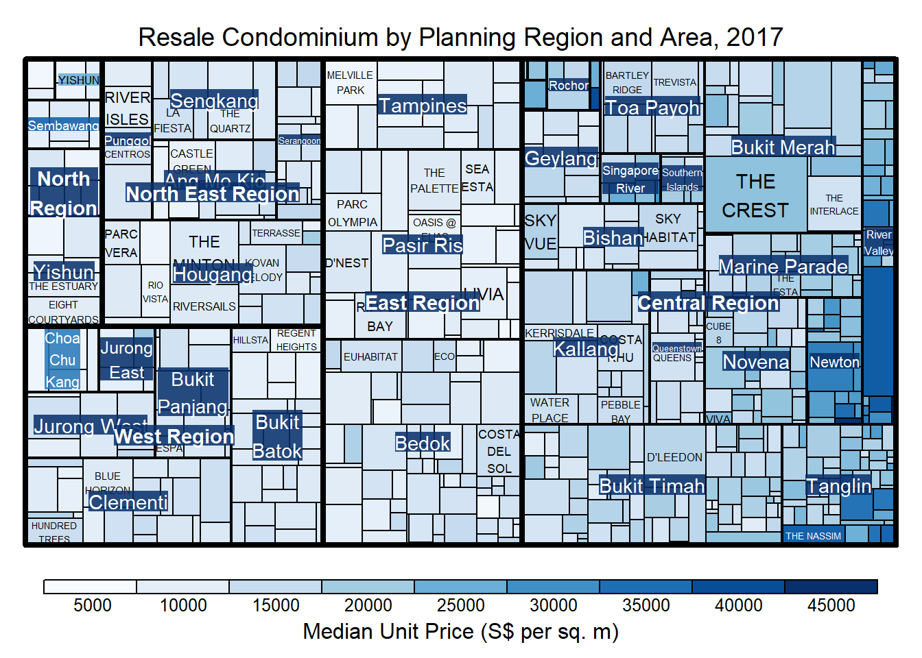
2.2 Designing Treemap using treemapify package

treemapify is a R package specially developed to draw treemaps in ggplot2.

2.2.1 Designing basic treemap

Show code

ggplot(data=realis2018_selected, 
       aes(area = `Total Unit Sold`,
           fill = `Median Unit Price ($ psm)`),
       layout = "scol",
       start = "bottomleft") + 
  geom_treemap() +
  scale_fill_gradient(low = "light blue", high = "blue")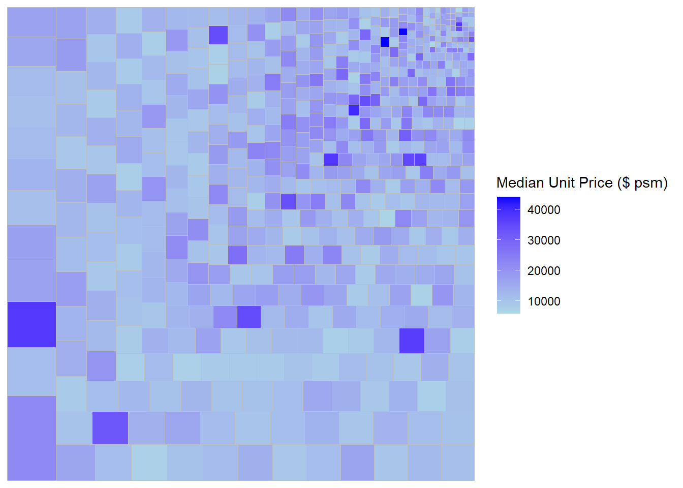

2.2.2 Defining hierarchy

Group by Planning Region

Use subgroup = Planning Region

Show code

ggplot(data=realis2018_selected, 
       aes(area = `Total Unit Sold`,
           fill = `Median Unit Price ($ psm)`,
           subgroup = `Planning Region`),
       start = "topleft") + 
  geom_treemap()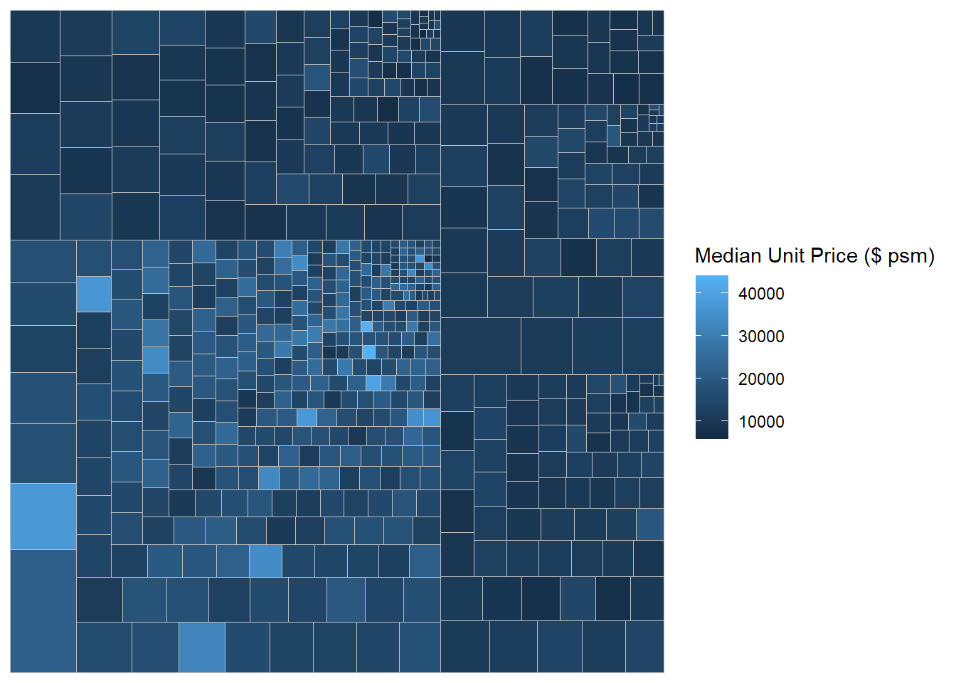

Group by Planning Area

Use subgroup = Planning Region & subgroup2 = Planning Area

Show code

ggplot(data=realis2018_selected, 
       aes(area = `Total Unit Sold`,
           fill = `Median Unit Price ($ psm)`,
           subgroup = `Planning Region`,
           subgroup2 = `Planning Area`)) + 
  geom_treemap()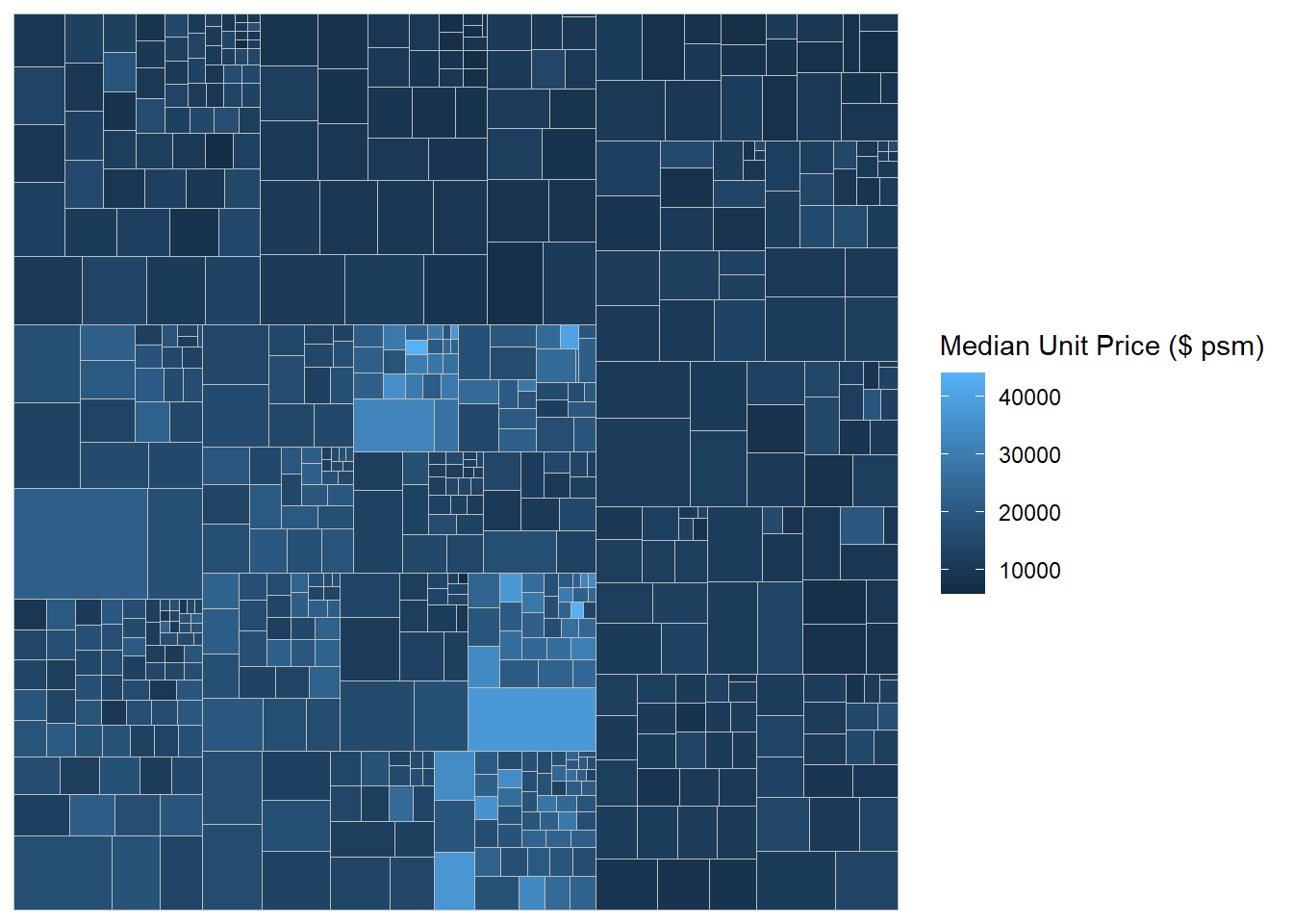

Add boundary line

Use geom_treemap_subgroup_border()

Show code

ggplot(data=realis2018_selected, 
       aes(area = `Total Unit Sold`,
           fill = `Median Unit Price ($ psm)`,
           subgroup = `Planning Region`,
           subgroup2 = `Planning Area`)) + 
  geom_treemap() +
  geom_treemap_subgroup2_border(colour = "gray40",
                                size = 2) +
  geom_treemap_subgroup_border(colour = "gray20")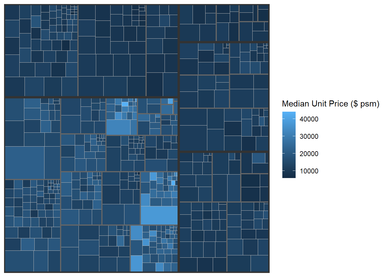

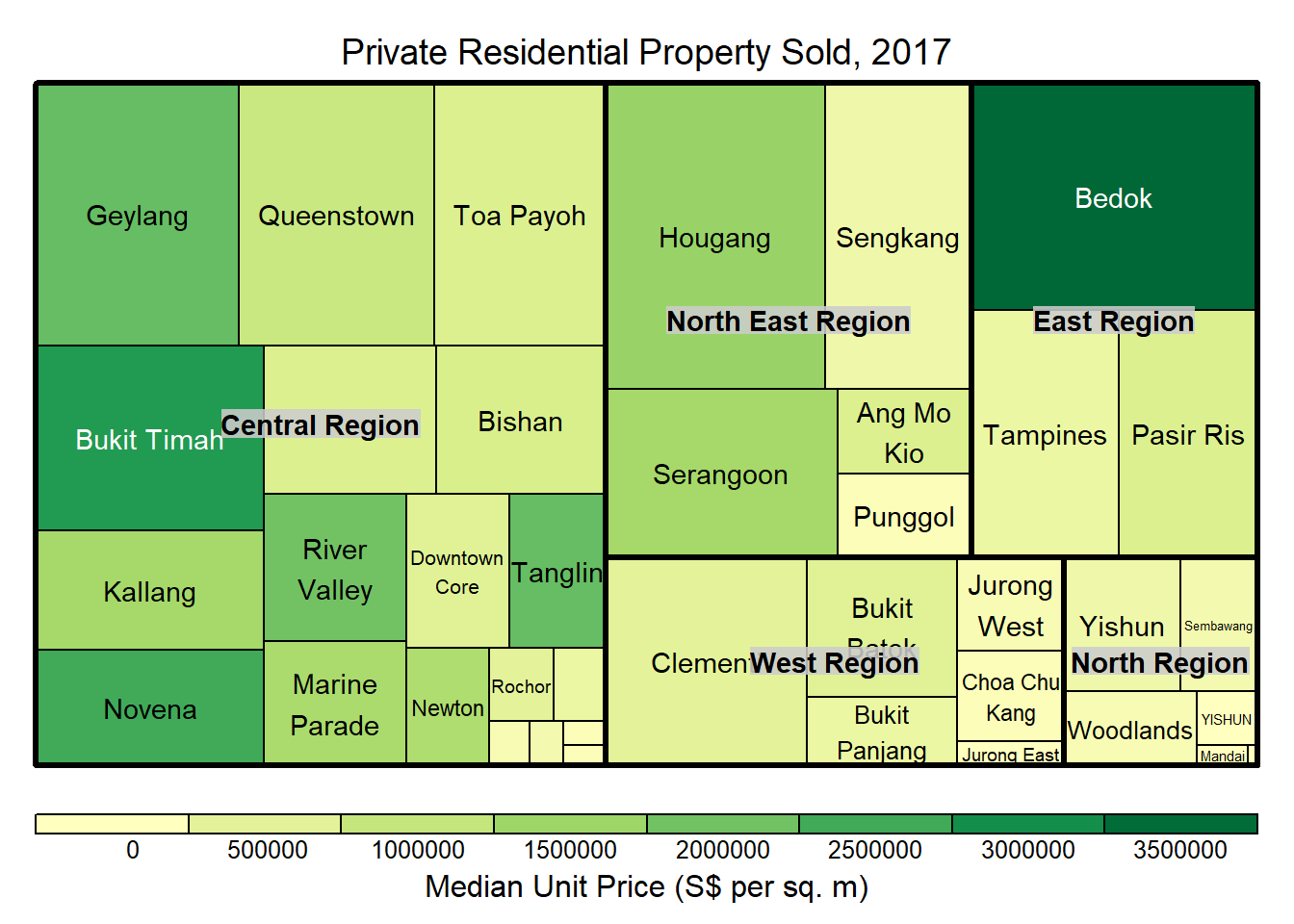
2.3 Designing Interactive Treemap using d3treeR

Use treemap() to build a treemap by using selected variables in condominium data.frame.

Show code

tm <- treemap(realis2018_summarised,
        index=c("Planning Region", "Planning Area"),
        vSize="Total Unit Sold",
        vColor="Median Unit Price ($ psm)",
        type="value",
        title="Private Residential Property Sold, 2017",
        title.legend = "Median Unit Price (S$ per sq. m)"
        )

Use d3tree() to build interactive treemap.

d3tree(tm,rootname = "Singapore" )

3. Self-exploratory on Singapore Consumer Price Index

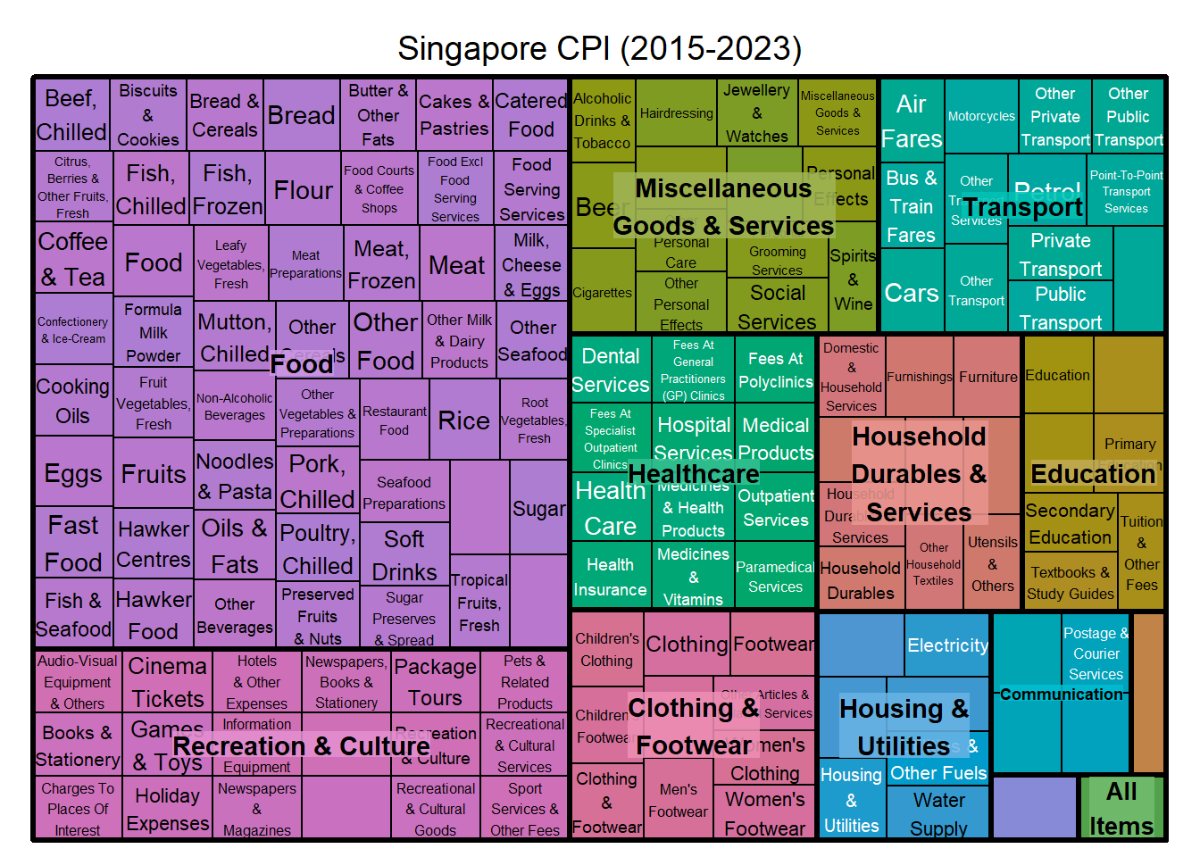
Import CPI data

The dataset (monthly CPI for the period between January 2015 to December 2023) is retrieved from Department of Statistics (DOS) Singapore.

pacman::p_load(tidyverse, treemap, treemapify, d3treeR, matrixStats)

Check on data structure of dataset

str(CPI)

colSums(is.na(CPI)) 

which(is.na(CPI))

Drop NA values

CPI2 <- na.omit(CPI)

str(CPI2)

Rename category variable

CPI3 <- CPI2 %>%
  rename(
  category =  `Data Series`
)

Group sub-categories into main categories

Show code

CPI4 <- CPI3 %>%
  mutate(
    main_category = case_when(
      # general
      row_number() %in% 1 ~ "All Items",
      row_number() %in% 2:55 ~ "Food",
      row_number() %in% 56:65 ~ "Clothing & Footwear",
      row_number() %in% 66:72 ~ "Housing & Utilities",
      row_number() %in% 73:82 ~ "Household Durables & Services",
      row_number() %in% 83:94 ~ "Healthcare",
      row_number() %in% 95:107 ~ "Transport",
      row_number() %in% 108:111 ~ "Communication",
      row_number() %in% 112:129 ~ "Recreation & Culture",
      row_number() %in% 130:136 ~ "Education",
      row_number() %in% 137:150 ~ "Miscellaneous Goods & Services",
      row_number() %in% 151 ~ "All Items Less Imputed Rentals On Owner-Occupied Accommodation",
      row_number() %in% 152 ~ "All Items Less Accommodation"
    )
  )


# shift main category column to 1st column
CPI4 <- CPI4[, c(ncol(CPI4), 1:(ncol(CPI4)-1))]

Prepare for CPI Treemap (Static)

Show code

CPI4_summarised <- CPI4 %>% 
  group_by(main_category,category) %>%
  summarise(`2023 Average` = rowMeans(CPI3[,c("2023 Dec", "2023 Nov", "2023 Oct", "2023 Sep", "2023 Aug", "2023 Jul",
                                     "2023 Jun", "2023 May", "2023 Apr", "2023 Mar", "2023 Feb", "2023 Jan")]),
            `2023 Max` = rowMaxs(as.matrix(CPI3[,c("2023 Dec", "2023 Nov", "2023 Oct", "2023 Sep", "2023 Aug", "2023 Jul",
                                     "2023 Jun", "2023 May", "2023 Apr", "2023 Mar", "2023 Feb", "2023 Jan")]))
            )

Show code

tm23 <- treemap(CPI4_summarised,
        index=c("main_category", "category"),
        vSize="2023 Average",
        vColor="2023 Max",
        title="Singapore CPI (2015-2023)",
        title.legend = "CPI"
        )

Prepare for CPI Treemap (Interactive)

Show code

d3tree(tm23, rootname = "Singapore CPI (2015-2023)", 
       value = paste("Max CPI : ", CPI4_summarised$`2023 Max`, 
              "\nAverage CPI : ", CPI4_summarised$`2023 Average`)
       )

4. References

16  Treemap Visualisation with R